


Field Oriented Control for servo drives
Field Oriented Control is a control method for electrical machines in which the control of torque and speed are directly based on the electromagnetic fields inside the electrical machine. FOC is very similar to the control of a DC machine. FOC is a technology to directly control the variables inside the machine, being of torque and flux. Thanks to decoupling of the stator currents into magnetizing flux current and torque producing current, the torque produced by the machine and the stator flux are controlled independently. Using a decoupled control, the magnetization flux inside the machine is maintained at the required level, and the torque can be controlled independently, to regulate the angular speed of the machine.
For high-performance motor applications, FOC is solely developed to allow smooth operation over a wide speed range, and to produce full torque at zero speed. FOC enables quick acceleration and deceleration of the drive by controlling the torque of the machine.
In this hands-on we primarily look at field oriented control for servo drives. Compared to traction, where maximum speed and power is an issue, in servo drives, position control becomes important. As explained in the book on drives, servo drives are cascaded drives with mainly three control loops.
- Position control
- Speed control
- Current control
All three control loops are build around a PI controller and the main structure is displayed below.
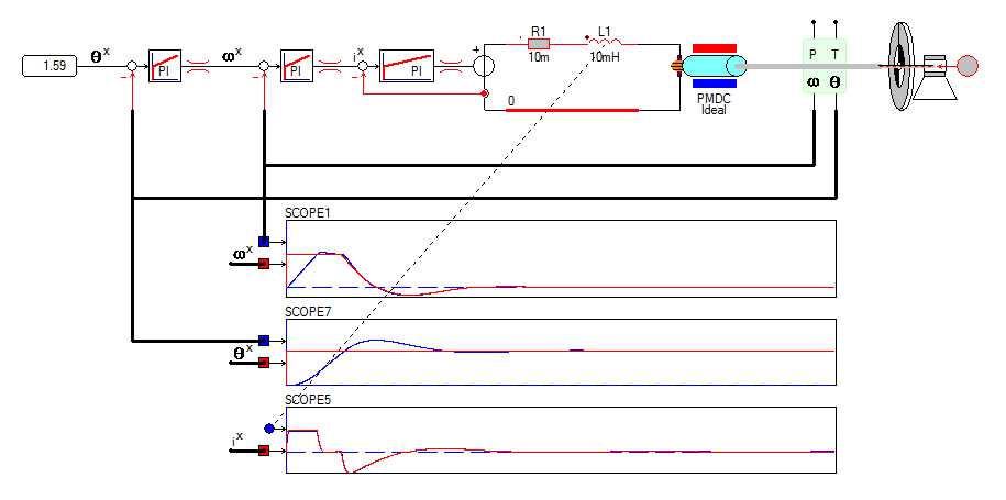
Here we will only look at the current loop. The examples shown above includes a DC motor. It seems that this is a simple solution, but the main reason for this and why we are finally going towards field oriented control is first briefly explained.
To better understand why we use FOC technique, we start with explaining the principle of the separately excited DC motor. In the DC motor, the control of the stator field and rotor field is done independently. The amplitude of the field current, or the size of the permanent magnets determines the strength of the flux. The current through the rotor windings amounts to how much torque the machine produces. The commutator on the rotor is important as it takes care that the current through the windings is such, that always torque is produced. Because of this mechanical commutator the torque production of the machine is nearly optimal for every rotor position. The trick is that the windings are switched by the commutator to keep the rotor flux orthogonal to the stator flux.
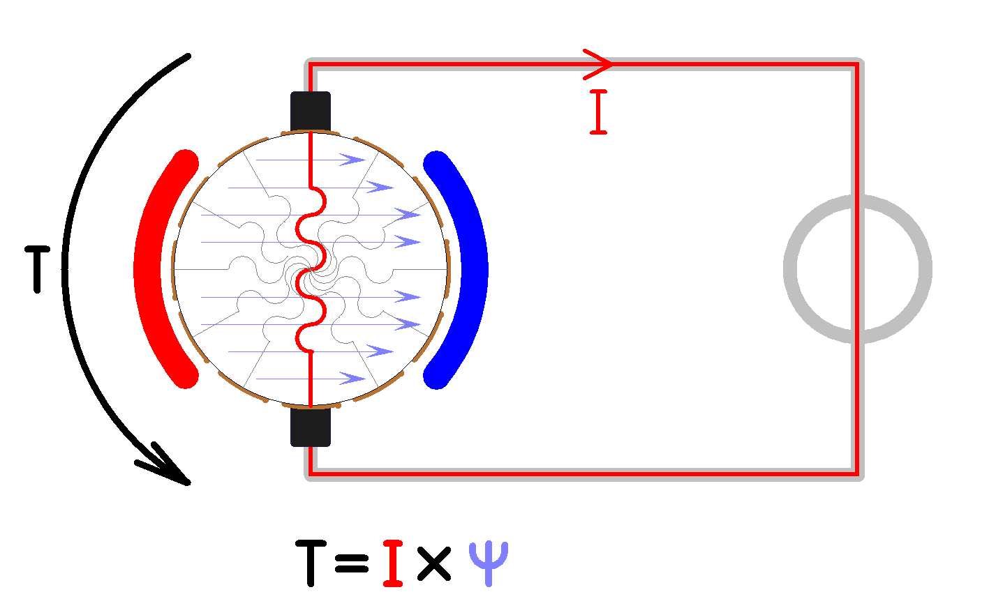
In a permanent magnet DC machine, the stator flux is constant and the rotor current is controlled. As a result the torque produced by the machine is linearly dependent on the stator current, no matter the position of the rotor.
Three phase AC servo motors have a different construction, as they do not have a mechanical commutator like the DC motor. For both the DC servo motor and the AC servo motor, only the stator currents can be controlled. In an AC servo motor, the rotor excitation is done by the permanent magnets mounted onto the shaft. The stator currents can be controlled and should be kept orthogonal to the rotor flux in order to produce maximum torque. This is the task of the field oriented control.
The main purpose of the field oriented control for synchronous and induction motors, is a separate control of the torque producing flux and the magnetizing flux. Although in a permanent magnet synchronous machine, the rotor flux is given by the magnets mounted on the rotor shaft, we can still influence that flux with the stator currents. In this way, the rotor flux can be increased or decreased, an important property when dealing with field weakening.
The figure below shows that the torque is produced as long as current and flux are 90 degrees out of phase.
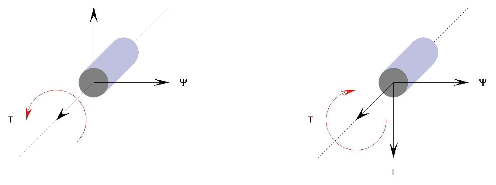
The goal is to imitate the mechanical commutator of the DC motor. The torque and the magnetizing flux components of stator current are decoupled by the foc. What this exactly means is that you will have two control signals that make the stator current. One signal controls the amount of magnetizing flux in the motor and the other signal controls the amount of torque producing flux. Together these two signals create a three phase current, which can be thought of as a combination of two currents. The magnetizing flux producing current is called Id and the torque producing current is called Iq. The subscripts d and q stem from the orientation of the current with respect to the rotor position. The d current is aligned with the magnetizing flux on the rotor. For a pmsm it is aligned with the magnetic field form the permanent magnets. This is called the "Langsachse" or "Direkte Achse", direct axis and indicated with the subscript d. The torque producing flux has to be orthogonal tot the magnetizing flux and is therefore called the "Quer Achse", orthogonal axis and indicated with the subscript q.
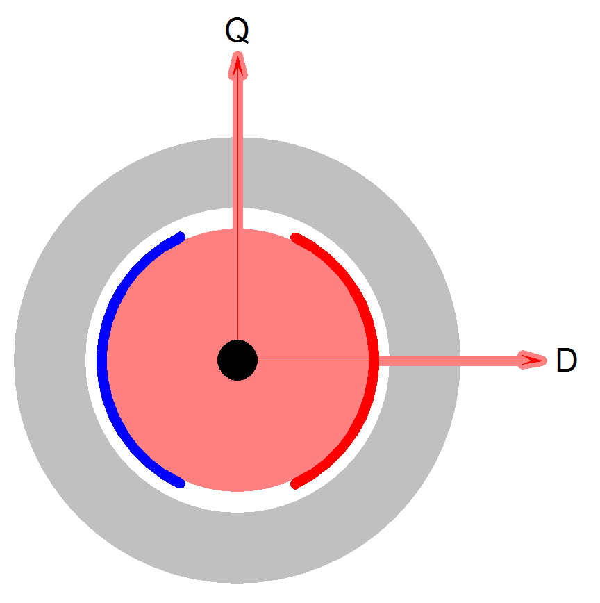
Thanks to the decoupled control of the magnetization flux, the torque producing stator flux can now be seen as an independent torque control. The decoupling of the torque and flux requires several mathematical transformations, and this is nowadays mostly done by microcontrollers.
The torque between rotor and stator is maximum, if the angle between the rotor field and stator field is 90 degrees. This is confirmed with a simulation where the current through phase a is held constant and the machine is slowly rotated. The torque produced by the machine is maximum at 90 degrees.
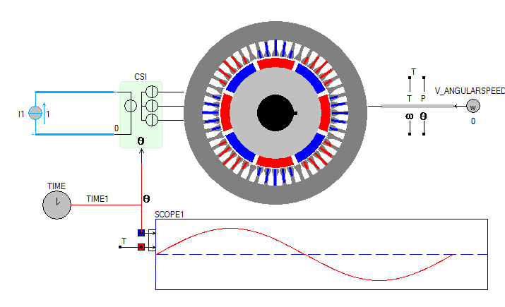
As can be seen in the above simulation, the rotor is held in a fixed position, while the current vector rotates around the machine. This will produce a torque that has a sinusoidal waveform depending on the rotor position. If the position of the current is 90 degrees ahead of the rotor, the produced torque is at its maximum. Same if the current vector is 90 degrees behind the rotor position, but now the produced torque is at its negative maximum.
How FOC works
In practice FOC of permanent-magnet synchronous motors starts by measuring two of three phase currents, ia and ib. Only two current sensors are needed as the third phase current is calculated from \(i_a + i_b + i_c = 0 \), however, mostly the three currents are measured seperatly in each inverter leg. So in the following we simply measure the three currents.
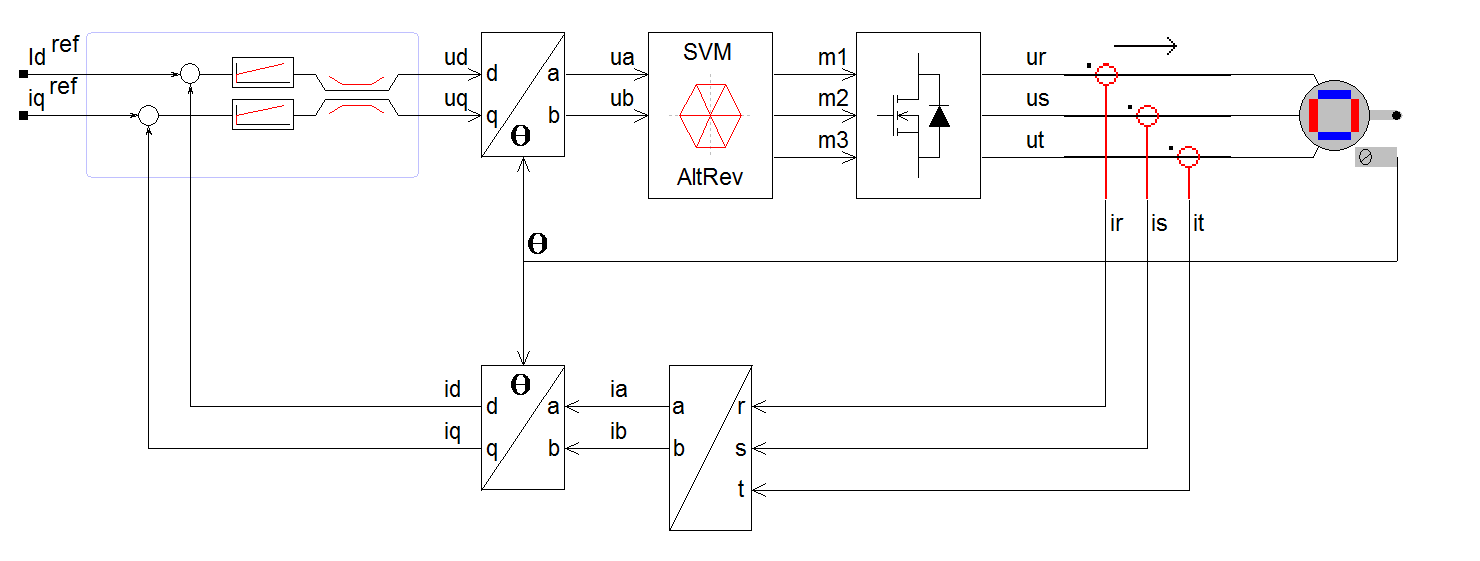
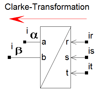
The currents iα and iβ are in the stationary reference frame, which means that the reference frame is fixed to the stator and standing still.
At this stage we could use the PI controller to control the stator voltage in order to get sinusoidal stator currents. However, this is not common practice because the bandwidth of hte PI should be very high to follow the angular pseedspeed of the stator currents. It is easier to apply a transformation and rotate the currents to steady state currents id and iq. Doing so, the bandwith of the PI controller can be much smaller since the currents id and iq are nearly steady state values.
To get the stready state currents id and iq, the currents iα and iβ are rotated to align with the rotor flux using the electrical angular position θ. The electrical angular position θ is in principle the angular position of the rotor flux. Because of the number of pole pairs pp, this electrical angular position is obtained by multiplying the mechanical angular position θm with the number of pole pairs pp.
\[\theta = pp \cdot \theta_m\]
The currents id and iq are obtained from the currents iα and iβ after the Park transformation. Both currents id and iq remain constant during steady-state conditions.
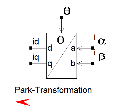
The currents id and iq are in a rotating reference frame, which means that the reference frame is rotating and aligned with the electrical angular position of the rotor flux and rotating with the same angular speed as the rotor.
The feedback control loop consists of a PI controller. It compares the currents id and iq with the reference currents, performs a Proportional-Integral [PI] control followed by a limiter.
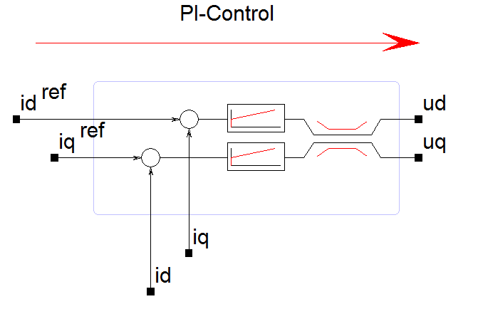
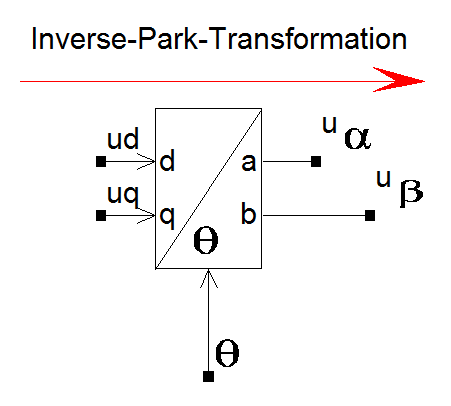
The output from the PI controller has to be transformed back into control signals for the inverter to actually build the motor voltages. The voltages ud and uq are rotated back into the stationary reference frame uα and uβ, using the same electrical angular position θ.
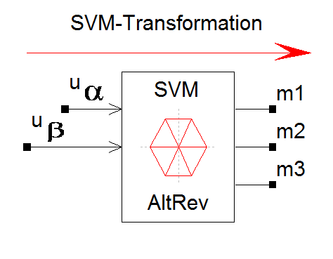
The control signals for the Mosfets in the inverter are then created using modulation. Mostly Space Vector Modulation [SVM] is choosen.
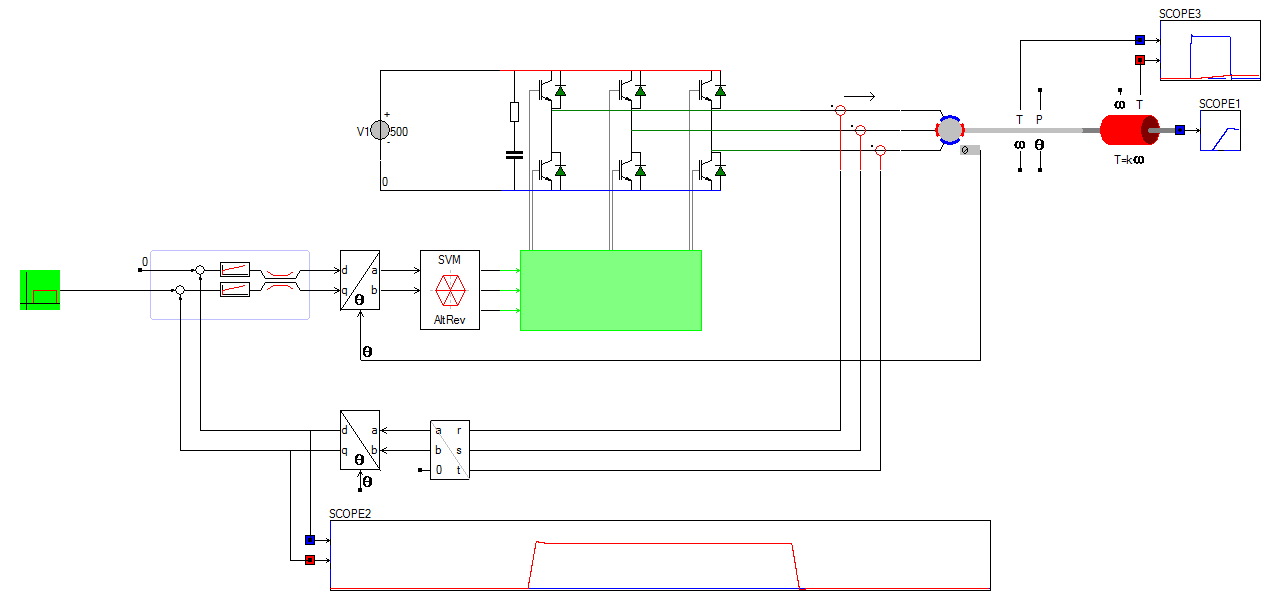
As can be seen from the simulation below, the torque produced by the motor is very close to the current iq reference current.
Mathematics of Field Oriented Control
To better understand the functioning of the above mentioned blocks, the mathematics behing field oriented control are given in this section. The mathematics is basically controlling the stator currents that are represented by a vector. The control of this current vector is based on vector operations that transform a three phase time and speed dependent system into a two coordinate (d and q axis) time invariant system. In other words, we describe the current in a three phase machine by two constant value, id and iq. Using those transformations the control is simplified and similar to that of a DC motor control. For FOC two constants are required as reference inputs;
- Torque reference current iq (aligned with the q axis)
- Flux reference current id (aligned with d axis)
The three-phase voltage, current and flux of an AC motor is described by a space vector. If we measure ia, ib, ic in the electrical machine as instantaneous currents in the stator phases, we can define a stator current vector as: \[ i_s= \begin{bmatrix} i_a\\i_b\\i_c \end{bmatrix} \] Where, [a, b, c] are the axes of a three phase system.
This current space vector is thus representing a three phase sinusoidal current. It has to be transformed into a time invariant orthogonal coordinate system. To do this, the transformation is divided into two steps:
- \([a, b, c] \rightarrow [α, β]\) (the Clarke transformation), which outputs a two coordinate time variant system.
- \([α, β] \rightarrow [d, q]\) (the Park transformation), which outputs a two coordinate time invariant system.
The \([a, b, c] \rightarrow [α, β]\) Clarke transformation is given as: \[ \begin{bmatrix} i_{\alpha}\\i_{\beta} \end{bmatrix} = \frac{2}{3} \begin{bmatrix} 1 & -\frac{1}{2} &-\frac{1}{2}\\ 0 & \frac{\sqrt{3}}{2} &-\frac{\sqrt{3}}{2}\\ \end{bmatrix} \begin{bmatrix} i_a\\i_b\\i_c \end{bmatrix} \]
Per definition we align the axis α and the axis a are along same direction and β is orthogonal to the α axis. This gives the following vector diagram:
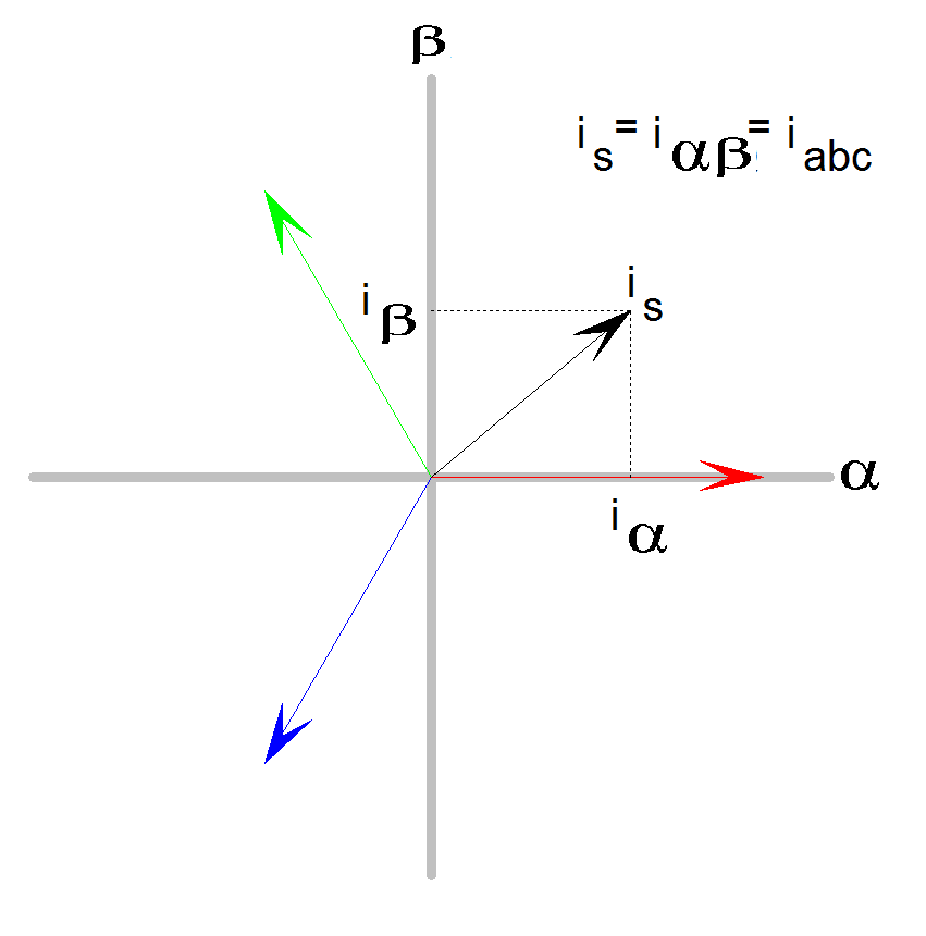
The \([α, β] \rightarrow [d, q]\) (Park transformation) is required to make the current vector look like a constant current. The Park transformation is the deciding one in the FOC. This transformation modifies the two phase fixed orthogonal system \((\alpha,\beta)\) into a \((d,q)\) rotating reference system. The transformation matrix is given below: \[ \begin{bmatrix} i_d\\i_q \end{bmatrix} = \begin{bmatrix} cos(\theta) & sin(\theta)\\ -sin(\theta) & cos(\theta) \end{bmatrix} \begin{bmatrix} i_{\alpha}\\i_{\beta} \end{bmatrix} \] where θ is the angle between the rotating \((d,q)\) and the fixed \((\alpha,\beta)\) coordinate system. This is the same rotation matrix known from vector analysis.
Consider the d axis aligned with the rotor flux. The relationship between the two reference systems for the current vector is shown below:
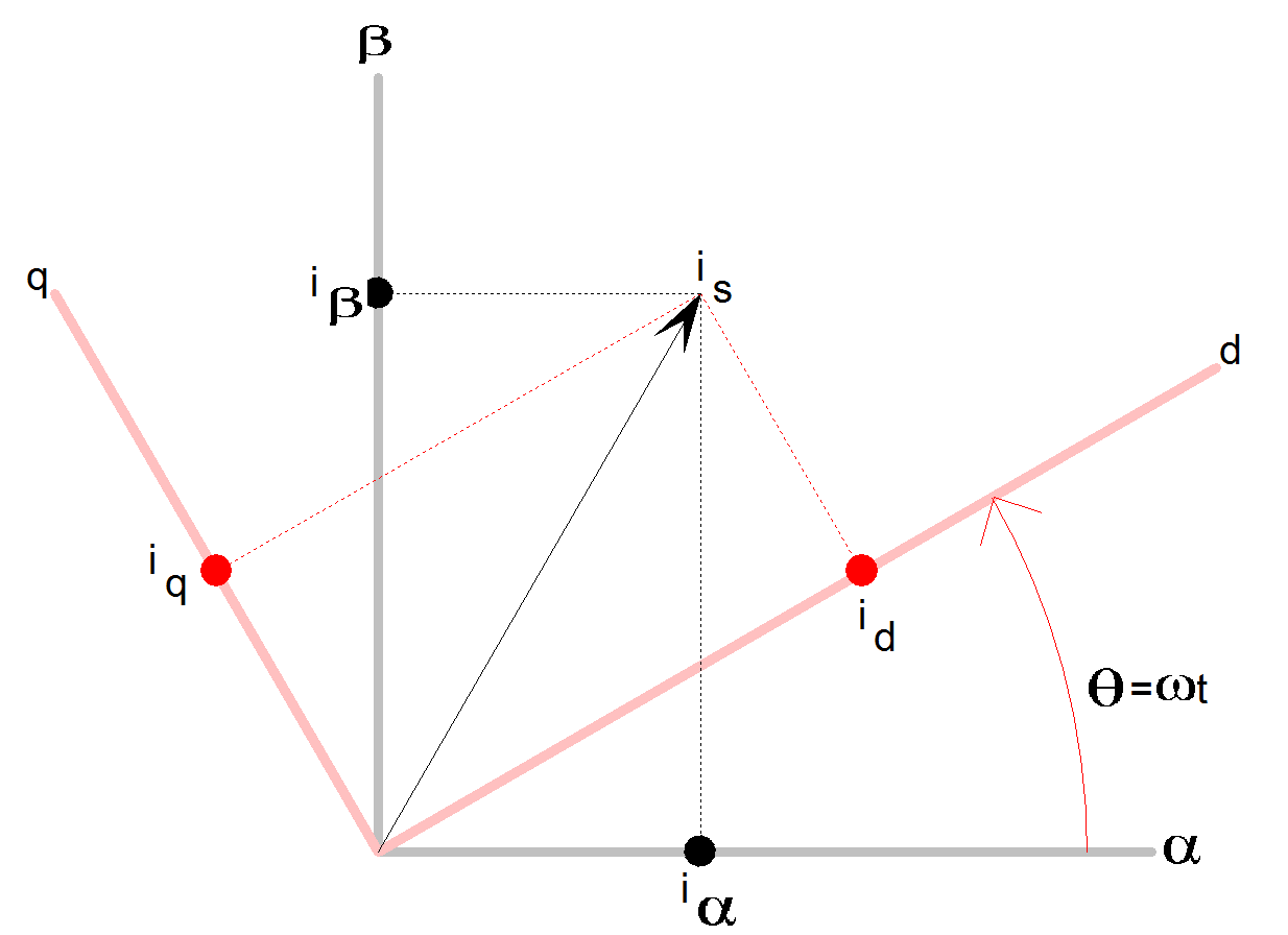
These torque and flux producing current components from the current vector are simply obtained from the current vector \((\alpha, \beta)\) and from the position of the rotor flux θ. By knowing the accurate rotor position, the current vector \([i_d,i_q]\) is easily calculated by using this rotation.
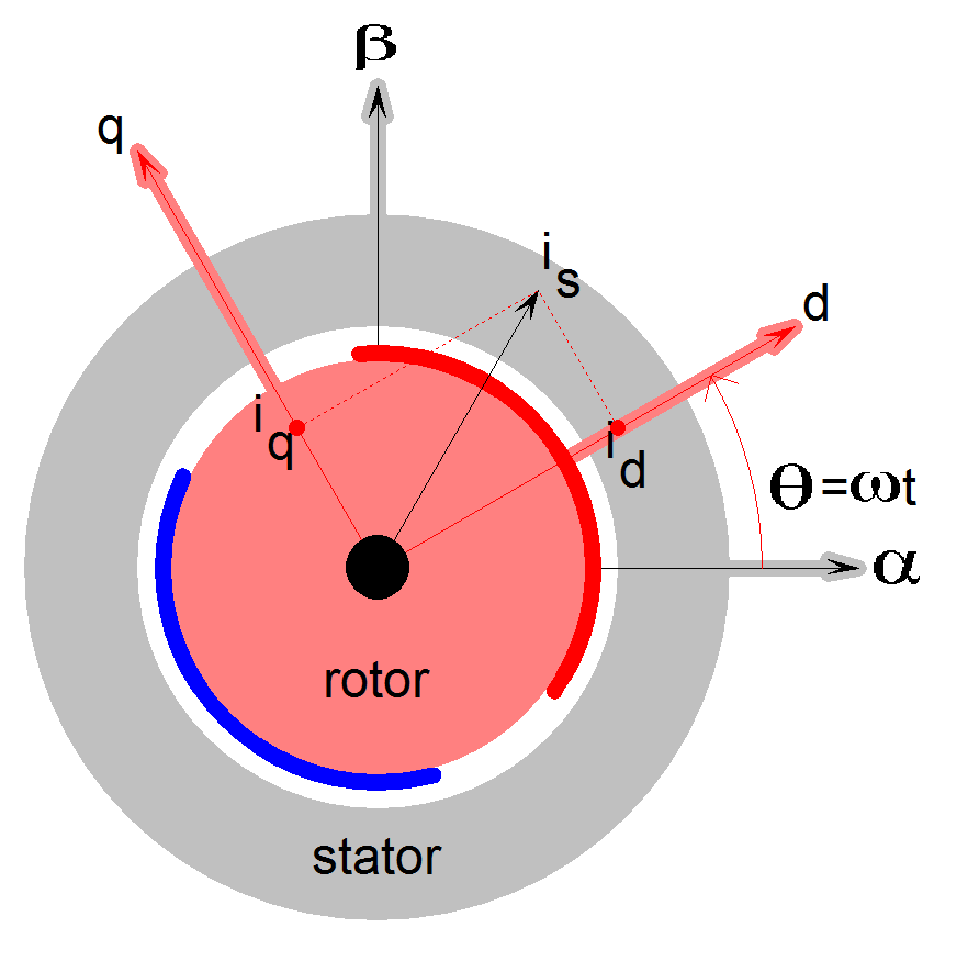
At this moment, the torque can be controlled directly using a PI controller, because flux component (id) and torque component (iq) are independent now. Using two PI controllers, we can calculated the voltage \([u_d,u_q]\) required to control the current inside the electric motor.
These voltages \([u_d,u_q]\) have to be transformed back into gating signals for the power electronics inverter in order to create the wanted current vector \([i_d,i_q]\). This is done by first using the inverse of the Park transformation, to rotate the voltage vector \([u_d,u_q]\) back from the rotating reference frame into the fixed reference frame by the angle -θ \[ \begin{align} u_{\alpha} &=u_d cos(\theta) &-u_q sin(\theta)\\ u_{\beta} &=u_d sin(\theta) &+u_q cos(\theta)\\ \end{align} \]
Since there is no hardware implementation for the inverse Clarke transformation other then power electronics, we have to use a modulation technique and a switched power electronics inverter to build the three phase voltage \([u_a, u_b, u_c]\). \[ \begin{bmatrix} u_a\\u_b\\u_c \end{bmatrix} = \begin{bmatrix} SVM\\Modulation \end{bmatrix} \begin{bmatrix} u_{\alpha}\\u_{\beta} \end{bmatrix} \] Mostly Space Vector Modulation [SVM] is chosen because it delivers a 15% higher output voltage compared to sine-triangular Pulse Width Mudulation [PWM]
Practical implementation of Field Oriented Control
With practical we mean the practical implemtation into a simulation model and/or implentation of the embedded control. There are a number of extra steps that have to be taken before we can apply the foc for torque, speed and/or position control.
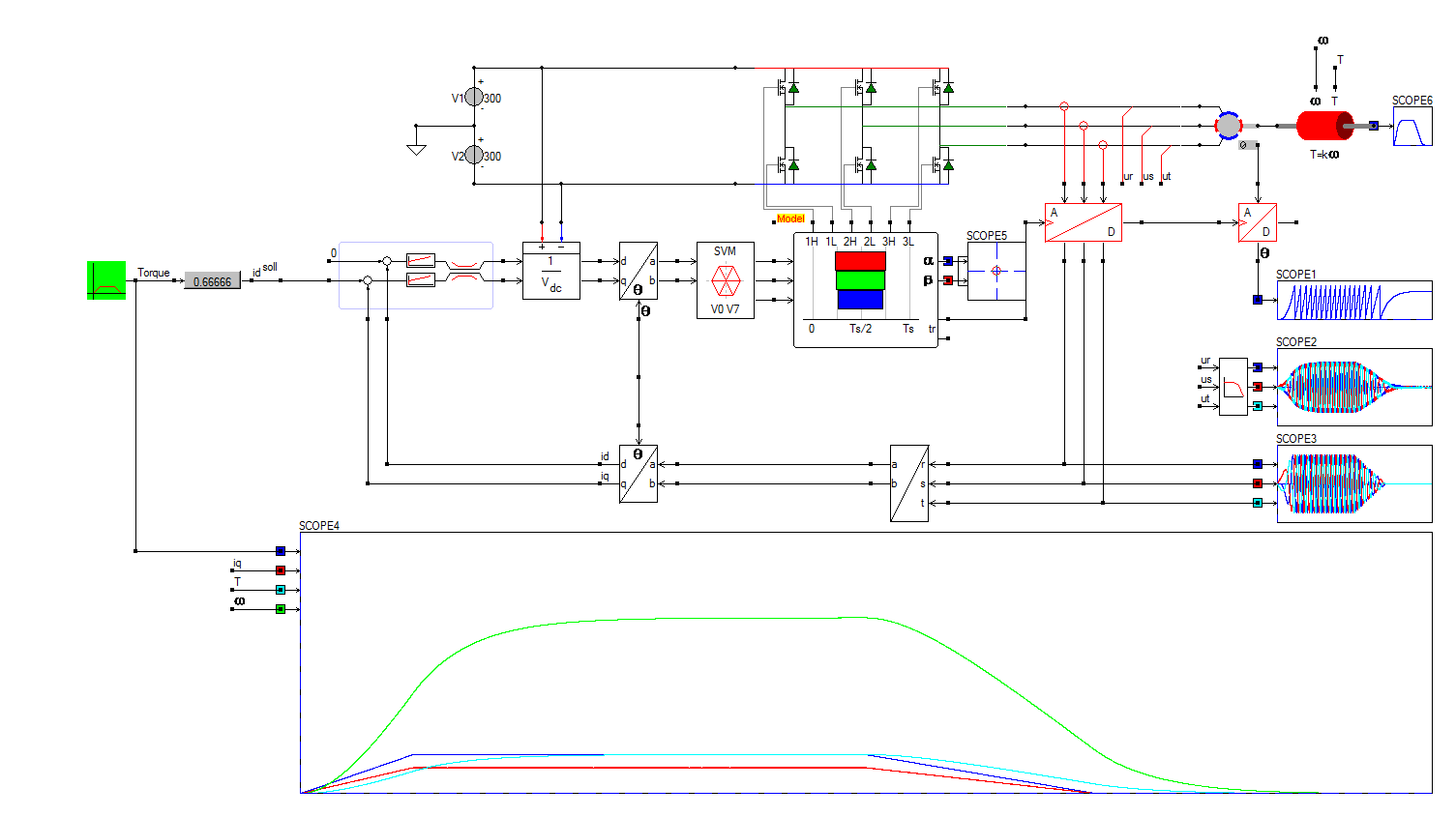
First the stator phase currents are measured. This is done using sensing resistors in the inverter, or by using hall sensors to measure the current in the three phase outputs from the inverter. In the simulation, the measurement of the currents in the outgoing lines of the inverter are preferred. Note the internal series resistance of the current sensor.
The measured currents are fed into the Clarke transformation block. The outputs of this transformation are the currents \(i_\alpha\) and \(i_\beta\). These two current components go into the Park transformation block that returns the current in the (d, q) reference frame. The \(i_d\) and \(i_q\) currents are compared to the reference currents: \(i_d^{ref}\) (the flux reference) and \(i_q^{ref}\) (the torque reference).
To study the influence of the sampling in digital systems, an analog to digital converter ADC can be used to sample the measured current. The trigger signal is produced by the modulator [PWM] or [SVM]. The trigger is either at the beginning, middle or at the end of a period. This depends on the type of modulation and control. (The modulation blocks in Caspoc provides two trigger signals for this purpose.)
If current sensing resistors are placed in the inverter legs, sampling should take place at the begin or end of the period. This ensures that current is measured at the moment that all low-side switches, if any, are closed. Analog RC filters are employed to remove any switching noise from the measured signals, but introduce a phase lag that has to be corrected inside the control algorithm.
The outputs of the PI controllers are the voltages \(u_d\) and \(u_q\). They are rotated back to the fixed reference frame using the inverse Park transformation. The outputs of this transformation are \(u_\alpha\) and \(u_\beta\), that are input to the space vector modulation [SVM] algorithm. The outputs of the space vector modulation algorithm gives the gate signals that drive the inverter.
To make the control independent of the DC link voltage, the outputs from the PI controllers are scaled to a unity signal. This is done by dividing the outputs from the PI controllers by the measured DC link voltage.
To avoid saturation of the controller and to avoid distortion of the output voltage, the output from the PI controllers is limited to the maximum voltage, the inverter can produce. In case of a sine-trangular pulse width modulation [PWM], the output form the PI controllers is limited to +/-1. In case of space vector modulation, the inverter can create a voltage vector that is 15% larger compared to pulse width modulation. Therefore the limit in the PI controller has to be set to 1.15 if space vector modulation is used.
To observe the voltage waveform that is "seen" by the electric machine terminals, the outputs from the voltage sensor can be made visible in a scope. As this would result in only a discrete signal alternating between the positive and negative DC link voltage, a low pass filter is applied. This filter will let only pass the basic harmonics, not the harmonics due to switching events. From this information the typical voltage waveform for space vector modulation can be deduced. The amplitude of the basic harmonic is visible and it can be verified agains the DC link voltage plus the extra 15%.
Both the Park and inverse Park transformations need the rotor flux position. This means that the rotor flux position is important and needs to be measured accurate. There various type of encoders to measure the rotor position and there are observers that can predict the rotor postion from the measured motor voltage and current.
![Angular position, modules 2π[Rad]<br>Click to close the image](CurrentControl2_SCOPE1.png "Angular position, modules 2π[Rad] [Click to view larger image]")
![Filtered output voltage[Volt]<br>Click to close the image](CurrentControl2_SCOPE2.png "Filtered output voltage[Volt] [Click to view larger image]")
![Output current[A]<br>Click to close the image](CurrentControl2_SCOPE3.png "Output current[A] [Click to view larger image]")
![Torque command in Nm[Dark blue], Commanded torque minus acceleration torque in load in Nm[Light blue], Current Iq[Red], Angular speed ω in Rad/s[Green]<br>Click to close the image](CurrentControl2_SCOPE4.png "Torque command in Nm[Dark blue], Commanded torque minus acceleration torque in load in Nm[Light blue], Current Iq[Red], Angular speed ω in Rad/s[Green] [Click to view larger image]")
The torque command is given to be \(40Nm\) from \(100ms\) to \(500ms\). The commanded torque minus the acceleration torque is the final load torque.
Changing the Space Vector Modulation
Changing the Space Vecotr Modulation from Centerlin into discontinuous, lowers the switching losses. The output voltage will be clamped to the DC bus voltage during the discontinuou period, as can be viewed in the filtered output voltage. The current remains sinusoidal as was with Centerline space vector modulation. The voltage harmonics are larger compared to centerline SVM.
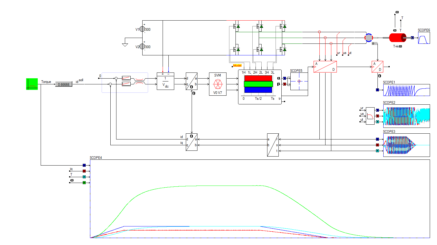
![Angular position, modules 2π[Rad]<br>Click to close the image](CurrentControl2_SVM4_SCOPE1.png "Angular position, modules 2π[Rad] [Click to view larger image]")
![Filtered output voltage[Volt] for SVM:method=4, Discontinouos space vector modulation. The output voltage is now held constant during a short period of time, meaning less switching losses, but different harmonics.<br>Click to close the image](CurrentControl2_SVM4_SCOPE2.png "Filtered output voltage[Volt] for SVM:method=4, Discontinouos space vector modulation. The output voltage is now held constant during a short period of time, meaning less switching losses, but different harmonics. [Click to view larger image]")
![Output current[A] for discontinuous space vector modulation remains sinusoidal.<br>Click to close the image](CurrentControl2_SVM4_SCOPE3.png "Output current[A] for discontinuous space vector modulation remains sinusoidal. [Click to view larger image]")
![Torque command in Nm[Dark blue], Commanded torque minus acceleration torque in load in Nm[Light blue], Current Iq[Red], Angular speed ω in Rad/s[Green]<br>Click to close the image](CurrentControl2_SVM4_SCOPE4.png "Torque command in Nm[Dark blue], Commanded torque minus acceleration torque in load in Nm[Light blue], Current Iq[Red], Angular speed ω in Rad/s[Green] [Click to view larger image]")
When the Space Vector modulation is changed from centerlin to discontinuous, the output voltage changes. The ouput current remains sinusoidal.
Practical implementation of Field Oriented Control with cascaded speed control
The next step is to add the speed control. The actual speed of the motor is captured at the load and since this is a slow varying signal, we are not sampling the motor speed.
A single PI controller is added to the previous simulation, which regulates the torque of the motor by setting the reference value for \(i_q\). The maximum current is limited to \(50\) Amperes and the gain and time constant of the PI controller are set inside the PIcontrol block.
In the simulation below the angular speed command is given to be \(90Rad/s\) from \(100ms\) to \(500ms\). Only the torque consumed by the rotating load is displayed in the scopes, being the commanded torque minus the acceleration torque. A constant load torque of \(20Nm\) is added to the drive shaft.
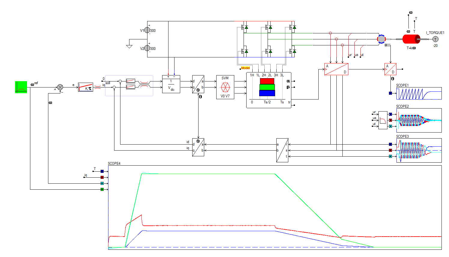
![Angular position, modules 2π[Rad]<br>Click to close the image](SpeedCurrentControl_SCOPE1.png "Angular position, modules 2π[Rad] [Click to view larger image]")
![Filtered output voltage[Volt]<br>Click to close the image](SpeedCurrentControl_SCOPE2.png "Filtered output voltage[Volt] [Click to view larger image]")
![Output current[A]<br>Click to close the image](SpeedCurrentControl_SCOPE3.png "Output current[A] [Click to view larger image]")
![Torque on the load(Excluding acceleration torque) in Nm[Dark blue], Current Iq[Red], Angular speed ω in Rad/s[Light blue], Reference angular speed ω in Rad/s[Green]<br>Click to close the image](SpeedCurrentControl_SCOPE4.png "Torque on the load(Excluding acceleration torque) in Nm[Dark blue], Current Iq[Red], Angular speed ω in Rad/s[Light blue], Reference angular speed ω in Rad/s[Green] [Click to view larger image]")
The angular speed command is given to be \(90Rad/s\) from \(100ms\) to \(500ms\). A constant load torque of \(20Nm\) is added to the drive shaft. The commanded torque minus the acceleration torque is the final load torque shown by the dark-blue trace.
The constant load torque of \(T_{hold} = 20Nm\) is clearly visible in the required current \(i_q\). Since \(K_e = 1\), the required holding current equals \[ i_q^{hold} = \frac{T_{hold}} { {2 \over 3} K_e } = 13.3A \]
Practical implementation of Field Oriented Control with cascaded speed and position control
Applying the cascaded position control requires the angular position of the shaft. A gearbox with ratio \(1:1\) is already included for future requirements. The mechancial angular position is simply the integral of the angular speed \[\theta_m = \int_0^\infty{\omega dt}\]
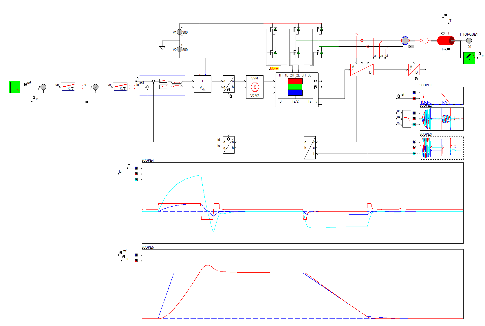
![Angular position, modules 2π[Rad]<br>Click to close the image](PositionSpeedCurrentControl_SCOPE1.png "Angular position, modules 2π[Rad] [Click to view larger image]")
![Filtered output voltage[Volt]<br>Click to close the image](PositionSpeedCurrentControl_SCOPE2.png "Filtered output voltage[Volt] [Click to view larger image]")
![Output current[A]<br>Click to close the image](PositionSpeedCurrentControl_SCOPE3.png "Output current[A] [Click to view larger image]")
![Torque on the load(Excluding acceleration torque) in Nm[Dark blue], Current Iq[Red], Angular speed ω in Rad/s[Light blue], Reference angular speed ω in Rad/s[Green]<br>Click to close the image](PositionSpeedCurrentControl_SCOPE4.png "Torque on the load(Excluding acceleration torque) in Nm[Dark blue], Current Iq[Red], Angular speed ω in Rad/s[Light blue], Reference angular speed ω in Rad/s[Green] [Click to view larger image]")
![Angular position of the shaft[Red] and reference angular position[Blue] in Radians.<br>Click to close the image](PositionSpeedCurrentControl_SCOPE5.png "Angular position of the shaft[Red] and reference angular position[Blue] in Radians. [Click to view larger image]")
The angular position reference command is given to be \(20Rad\) from \(100ms\) to \(500ms\). A constant load torque of \(20Nm\) is added to the drive shaft. The commanded torque minus the acceleration torque is the final load torque shown by the dark-blue trace in Scope 4.
Practical implementation of Field Oriented Control with cascaded speed and position S-curve control
To improve the dynamics of the control, the angular position reference command is given by the Profile block. This profile block calculates the dynamic references need to get a S-curved position. From the required angular position, the required acceleration is calculated, from which the required angular speed and angular position is calculated using two integrator blocks. This angular position reference is used as reference for the position control.
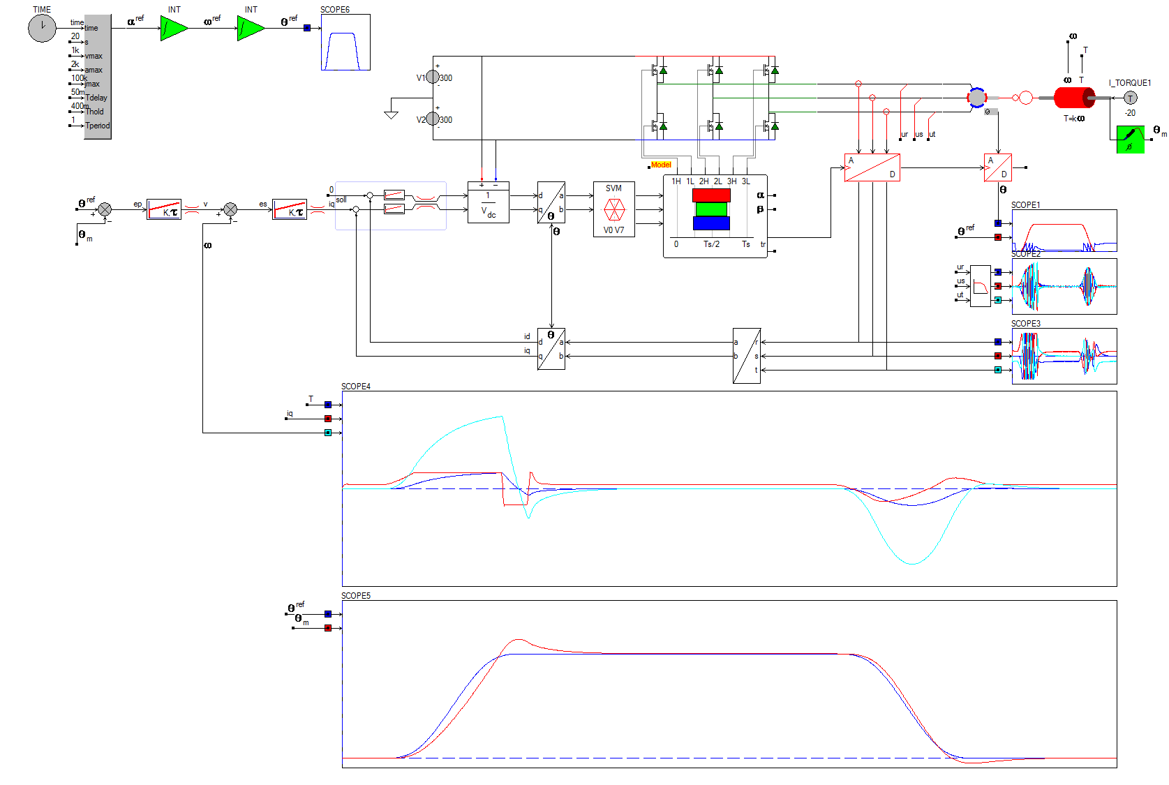
![Angular position, modules 2π[Rad]<br>Click to close the image](ProfilePositionSpeedCurrentControl_SCOPE1.png "Angular position, modules 2π[Rad] [Click to view larger image]")
![Filtered output voltage[Volt]<br>Click to close the image](ProfilePositionSpeedCurrentControl_SCOPE2.png "Filtered output voltage[Volt] [Click to view larger image]")
![Output current[A]<br>Click to close the image](ProfilePositionSpeedCurrentControl_SCOPE3.png "Output current[A] [Click to view larger image]")
![Torque on the load(Excluding acceleration torque) in Nm[Dark blue], Current Iq[Red], Angular speed ω in Rad/s[Light blue], Reference angular speed ω in Rad/s[Green]<br>Click to close the image](ProfilePositionSpeedCurrentControl_SCOPE4.png "Torque on the load(Excluding acceleration torque) in Nm[Dark blue], Current Iq[Red], Angular speed ω in Rad/s[Light blue], Reference angular speed ω in Rad/s[Green] [Click to view larger image]")
![Angular position of the shaft[Red] and reference angular position[Blue] in Radians.<br>Click to close the image](ProfilePositionSpeedCurrentControl_SCOPE5.png "Angular position of the shaft[Red] and reference angular position[Blue] in Radians. [Click to view larger image]")
The angular position reference command is given by the Profile block. From the required angular position, the required acceleration is calculated, from which the required angular speed and angular position is calculated using two integrator blocks. This angular position reference is used as reference for the position control. A constant load torque of \(20Nm\) is added to the drive shaft. The commanded torque minus the acceleration torque is the final load torque shown by the dark-blue trace in Scope 4.
The main difference with the previous simulation is the improvement of the angular position control since the S-curved angular position reference is easierer to follow. Still the drive is operated at its maximum limits, as can be seen at the maximum current.
Classification of Field Oriented Control
The observation of the rotor flux position is different if we consider the synchronous/pmsm or induction motor. In the first place, the field oriented control has an advantage: it can be used to control either synchronous or induction machines by simply changing the flux reference and rotor flux position observer. This easily eliminates one of the major shortcomings of the “classic” control structures: the portability from asynchronous to synchronous drives.
- In case of permanent magnet synchronous motor, the rotor flux is fixed and aligned with the magnets on the rotor, so there is no need to create any extra magnetising flux using the stator currents. Therefore, while controlling a PMSM, \(i_d^{ref}\) should be equal to zero. The rotor flux position is directly determined by a position sensor.
- Induction motors need a rotor flux that is created by the stator current. Therefore the flux reference \(i_d^{ref}\) in an induction motor drive should not be equal to zero. The rotor speed is not equal to the rotor flux speed because of slip. Therefore the rotor flux position has to be determined from the mechanical angular speed and the slip. .
FOC for pmsm is the easiest, as it only requires a position sensor for the rotor. There is a major difference between foc for traction and servo drives. For servo drives, the actual position of the rotor is required at any time instant. Therefore an encoder is used to get the absolute rotor position. For traction drives and drives where the absolute position is not important, a sensorless approach can be used. Here the rotor position is obtained from the motor voltages and currents. Various approaches exist but is beyond the scope of this text.
For the induction motor drive, foc can be classified into two types: Indirect IFOC and Direct DFOC schemes.
- In DFOC, the rotor flux vector is either measured by means of a flux sensor mounted in the air-gap or by using an observer measuring based on the machine equations and measurement of machine voltage and currents.
- For IFOC, the rotor flux vector is estimated using the mathematical current model of hte induction machine together with the measured a rotor speed.
Advantages of Field Oriented Control
- Improved torque response.
- Torque control at low frequencies and low speed.
- Dynamic speed accuracy.
- Reduction in size of motor, cost and power consumption.
- Four quadrant operation.
- Short-term overload capability.